Introduction:
It is well known that the Fourier transform of a signal's power spectrum is the auto-correlation function (Wiener Khinchin theorem). Therefore if we run a signal through an FFT, calculate the magnitude, and run a final FFT we have a particularly fast way of calculating auto-correlations. Since there are nice USRP GNU Radio FFT examples such as usrp_fft.py making use of the fftsink.py component it seemed like a reasonable afternoon project to add an auto-correlation window.
We started with a copy of fftsink.py, removed the windowing, extended the signal flow with a second FFT and a second magnitude calculation, redid the range labels, cut out the redundant data display half, and viola... with exception of some items such as proper normalization we have a working fast auto-correlation sink. We then modified usrp_fft.py to display the resulting fast auto-correlation in addition to the user selected FFT/scope/waterfall display.
The maximum auto-correlation is directly proportional to FFT length; thus the FFT length was extended out to 32768 bins which was about the maximum possible that the host computer could handle. The auto-correlation window update rate was changed to twice a second to help ease the computational burden yet still provided a near real time display; this change also required a modification of the fftsink.py display averaging time constant.
Sample
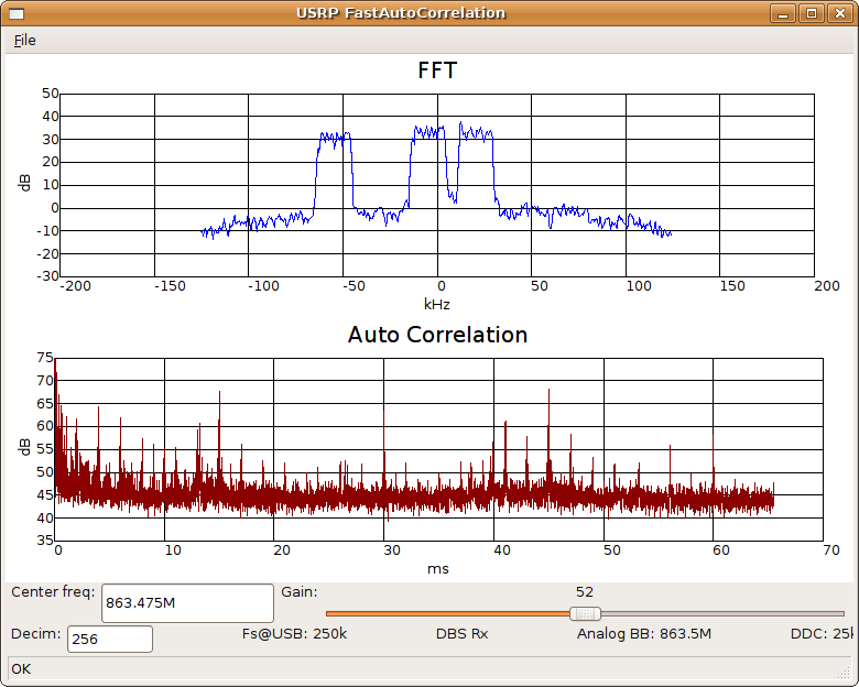
Screenshot - CDMA
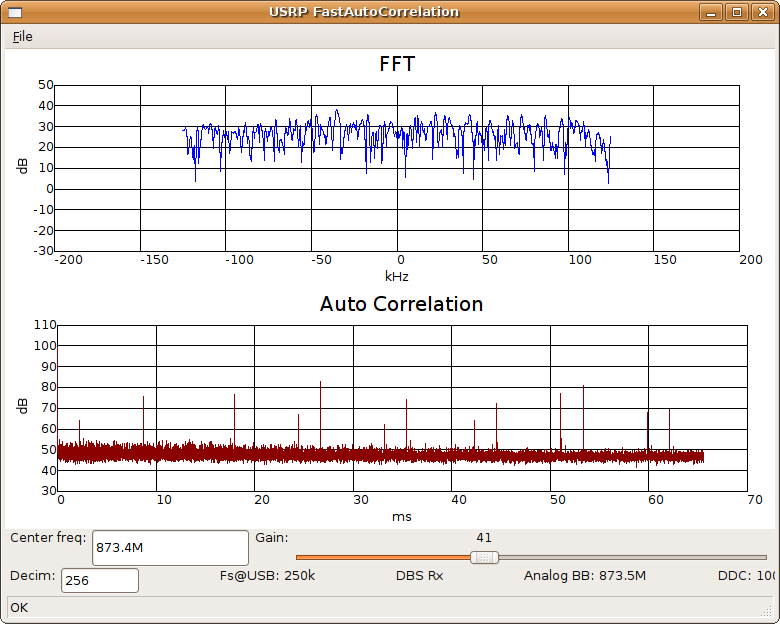
The screenshot above shows a slice of a
cellular telephone CDMA
signal. It should be noted that the entire CDMA actually spans
just over one megahertz yet here we have sampled just 250
kilohertz. Nonetheless very sharp and clearly defined correlation
peaks are visible which are characteristic of the CDMA system.
Same cell auto-correlation peaks are expected at ~26ms separations with
additional peaks presumably coming from other cells.
The narrowest spectrum window possible (USRP decimation rate = 256) was chosen to display the longest auto-correlation period (out to 64 ms with the 32768 point FFT). Lower decimation rates may be selected but will shorten the maximum auto-correlation time (e.g. a decimation rate of 16 would only give 4ms of data).
The narrowest spectrum window possible (USRP decimation rate = 256) was chosen to display the longest auto-correlation period (out to 64 ms with the 32768 point FFT). Lower decimation rates may be selected but will shorten the maximum auto-correlation time (e.g. a decimation rate of 16 would only give 4ms of data).
Sample
Screenshot - GPS L1 Signal
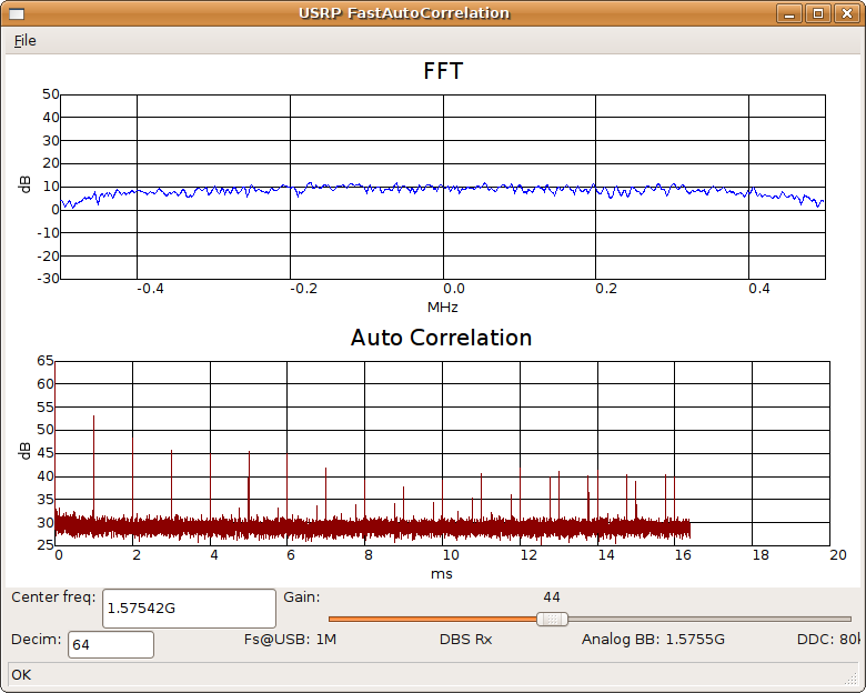
Another spread spectrum example:
An external GPS antenna / preamp
was
connected to the USRP and tuned to the GPS L1 frequency.
Artifacts from the circular auto correlation are quite
evident. No
signal is apparent in the FFT window while the auto correlation window
clearly indicates the presence of something with a 1 ms
periodicity. And indeed GPS C/A signals are in fact spread at a
1.023 MHz chip rate with cyclic 1023 bit long codes resulting in 1
ms cycles; data is transmitted at 50 baud or 20 ms per bit which
means odds are quite high that any given 1 ms chunk is a repetition of
the previous 1 ms.
The GPS signal spectrum is actually a little wider than shown above. The decimation rate of 64 was selected just to make the auto correlation graph a little prettier; lower decimation rates such as 16 will span the entire bandwidth but the auto correlation peaks then line up exactly with grid lines and become hard to see. But just for completeness we show what things look like when we cover the entire GPS C/A signal spectrum:
The GPS signal spectrum is actually a little wider than shown above. The decimation rate of 64 was selected just to make the auto correlation graph a little prettier; lower decimation rates such as 16 will span the entire bandwidth but the auto correlation peaks then line up exactly with grid lines and become hard to see. But just for completeness we show what things look like when we cover the entire GPS C/A signal spectrum:
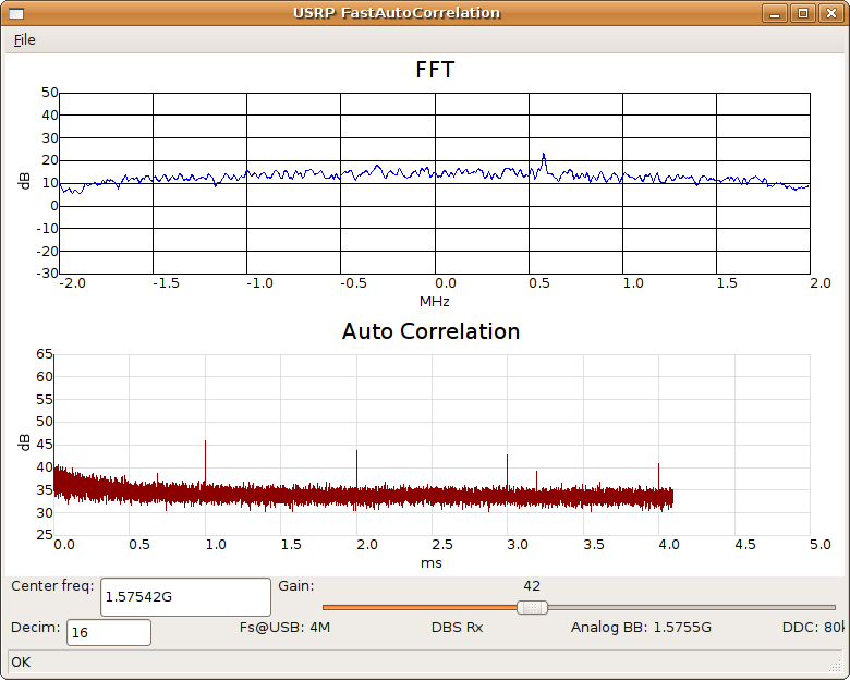
Above: Auto-correlation covering ±2MHz of GPS L1 frequency. The FFT spectrum does not show any evidence of the GPS signal (the spectrum is not entirely flat due to windowing and filtering; the small peak at 1576 MHz is an unrelated spur). On the other hand the auto-correlation clearly shows GPS signals as evidenced by 1 ms auto-correlation peaks. Grid color changed from black to light gray for clarity.
Sample
Screenshot - Motorola 3600 Baud Trunked Radio Control Channel
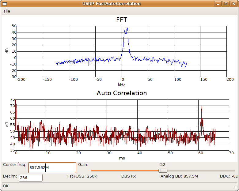
Here we sample a Motorola 3600 Baud trunked radio system. We note a strong auto-correlation peak at a little over 60 ms which presumably tells us something about the periodicity of the transmitted data.
Here we sample a Motorola 3600 Baud trunked radio system. We note a strong auto-correlation peak at a little over 60 ms which presumably tells us something about the periodicity of the transmitted data.
Sample
Screenshot - Motorola iDEN
And finally... Motorola's iDEN format as
used by companies such as
Southern Linc and Nextel. In this screenshot there are 3 active
iDEN channels visible; each channel consists of four 16QAM signals
which accounts for the nice broad flat spectrum peaks. The
auto-correlation
seems to show TDMA slots of 15ms which accounts for the strong peaks at
15 and 45 ms. Synchronization symbols transmitted every two
milliseconds also noticeably contribute to the auto-correlation
structure. To truly appreciate this modulation scheme one
should refer to U.S. Patents 6,909,761;
6,873,614; and 5,519,730.
The
GNU Radio Code:
If you have a fully functional GNU Radio and USRP installation you may wish to try things out for yourself. You will need:
All the usual usrp_fft.py and fftsink.py options and functions are available. You will probably need to make use of some of these features to adjust the fast auto-correlation reference level (especially since it is not normalized), dB per division, et cetera. Right click on the graph to see all available fast auto-correlation adjustment options. All the usual command line options are available as well.
Some tweaking pointers:
If you have a fully functional GNU Radio and USRP installation you may wish to try things out for yourself. You will need:
- usrp_fac.py (Modified GNU Radio usrp_fft.py component)
- facsink.py (Modified GNU Radio fftsink.py component)
All the usual usrp_fft.py and fftsink.py options and functions are available. You will probably need to make use of some of these features to adjust the fast auto-correlation reference level (especially since it is not normalized), dB per division, et cetera. Right click on the graph to see all available fast auto-correlation adjustment options. All the usual command line options are available as well.
Some tweaking pointers:
- The fast auto-correlation FFT length is set by parameter fac_size at line 111 in usrp_fft.py. You may adjust this up or down to better match your specific computational resources.
- The screen update rate set by the parameter at line 32 of facsink.py. This also may adjusted to better suit specific requirements.
Some Closing Comments:
One may well ask of what use is the auto-correlation?
It provides another way of visualizing data that brings out temporal features that may be obscured or lost in a FFT spectrum display.
For example, spread spectrum transmissions that may not be evident in an FFT display may pop up with strong auto-correlation spikes provided the spreading function is well correlated, the transmitted data is well correlated, and one is displaying an appropriate time span. Case in point - see above GPS example.
It can also provide additional details about transmitted signal periodicity that are not evident in an FFT display, such as in the trunked radio control channel screenshot. This may aid in an initial signal assessment but of course more serious analyses are only undertaken on the demodulated data stream itself.
If nothing else the auto-correlation makes for some pretty graphs.
Variations on the theme:
We may take the logarithm of the spectrum before the second FFT to produce the cepstrum. We use either the complex spectrum or the spectrum magnitude depending on whether we want the complex or real cepstrum. The end result does not provide information qualitatively different from the auto correlation and thus we do not present any cepstral analysis results.
These methods can also be applied to calculate cross-correlations as might be done in the search for certain signals with known characteristics.
Not so fast...
One should at all times remember the FFT (and this fast auto-correlation by extension) assumes that the signal is cyclic relative to the sampling window. Because your actual signal is not really the same sampled window repeating over and over again certain artifacts can be introduced. Some steps could be taken to overcome this such as doubling the data length with zero padding to eliminate cyclic data wrap around but this creates some other issues... in the end it easier to stick with the simplicity and speed of the cyclic fast auto-correlation.
Back to radiorausch home page